Overview
A 4-element phased-array Doppler radar system using HB100 microwave modules (10.525 GHz) with an ESP32-S3 firmware data collector and Raspberry Pi 4 host processor. The system employs custom signal conditioning with op-amp amplification, virtual ground biasing, and precision filtering to overcome the challenges of low-signal-level IF outputs. Two parallel processing pipelines enable both phase-coherent angle-of-arrival estimation (MUSIC algorithm) and amplitude-based zone classification robust to oscillator drift, with extended Kalman filtering for multi-target tracking.
Quick Summary
-
A 4-channel 10.525 GHz Doppler radar array using independent HB100 modules with custom analog signal conditioning.
-
Firmware (ESP32-S3) performs continuous 12-bit ADC sampling at 10 kHz per channel via DMA, streaming raw data blocks over USB-CDC to a host processor.
-
Host processor (Raspberry Pi 4) can run two different processing pipelines: a MUSIC-based speed and direction estimator (requires phase coherence via careful hardware design) and an amplitude-based zone classifier (robust to LO drift).
-
Custom MCP6002 op-amp configuration provides 1092× total gain (52× + 21×) across two stages with virtual ground biasing to handle bipolar IF signals on a unipolar ADC supply.
-
Extended Kalman Filter tracks target state (position, velocity) from speed and angle measurements with adaptive noise covariance.
-
Element spacing (37–38 mm center-to-center) gives ~0.112 m max baseline for 10.525 GHz carrier (λ ≈ 28.5 mm).
Key Features
-
4-channel receiver array with independent HB100 Doppler modules, each with its own free-running Gunn oscillator (10 µV–2 mV IF output typically at ~200 Hz nominal Doppler).
-
Analog signal conditioning: MCP6002 dual op-amp provides 1092× total amplification in two stages (52× non-inverting, then 21× inverting) with virtual ground set to ESP32-S3's 1.65 V rail reference.
-
Multi-stage LPF design: 5 V supply bypass filtering (three 10 Ω resistors in parallel with 10 µF + 100 µF + 0.1 µF caps), pre-op-amp EMI filtering (10 µF || 10 kΩ to virtual ground), and final bandwidth limiting (2 kΩ + 100 nF to real ground, ~800 Hz cutoff).
-
Dual processing pipelines:
- Radar Processor (radar_processor.py): DC removal → 4th-order Butterworth bandpass (10–800 Hz) → Hanning windowed FFT (1024-point) → peak Doppler bin detection → phase extraction → MUSIC pseudospectrum → EKF state tracking.
- Zone Classifier (zone_classifier.py): Same front-end DSP but skips phase processing; uses per-channel FFT magnitudes at common Doppler peak for monopulse-based left/right bias estimation and 5-zone classification (FAR_LEFT, LEFT, CENTER, RIGHT, FAR_RIGHT).
-
12-bit ADC @ 10 kHz per channel, 1024-sample blocks (~102.4 ms coherency windows), 0xDEADBEEF sync word framing.
-
Extended Kalman Filter for continuous target tracking with state [x_m, y_m, v_x, v_y] and adaptive observation noise tuning.
Tools Used
- Raspberry Pi 4 Model B (4 GB RAM) — Host processor
- ESP32-S3-DevKitC-1 — Firmware platform (USB-CDC, ADC DMA, FreeRTOS)
- 4× HB100 Doppler modules (10.525 GHz, 10 µV–2 mV IF output)
- MCP6002 dual op-amp (rail-to-rail input/output, ±3.3 V)
- Passive components: resistors, capacitors (10 µF, 100 µF, 0.1 µF, 100 nF), 10 kΩ resistor (virtual ground divider)
- Python 3.9+, NumPy, SciPy (Butterworth filters, FFT, linear algebra for MUSIC)
- C (ESP-IDF 5.1+), FreeRTOS, ADC continuous mode DMA
Images
Circuit Diagram - Signal Conditioning and Amplification
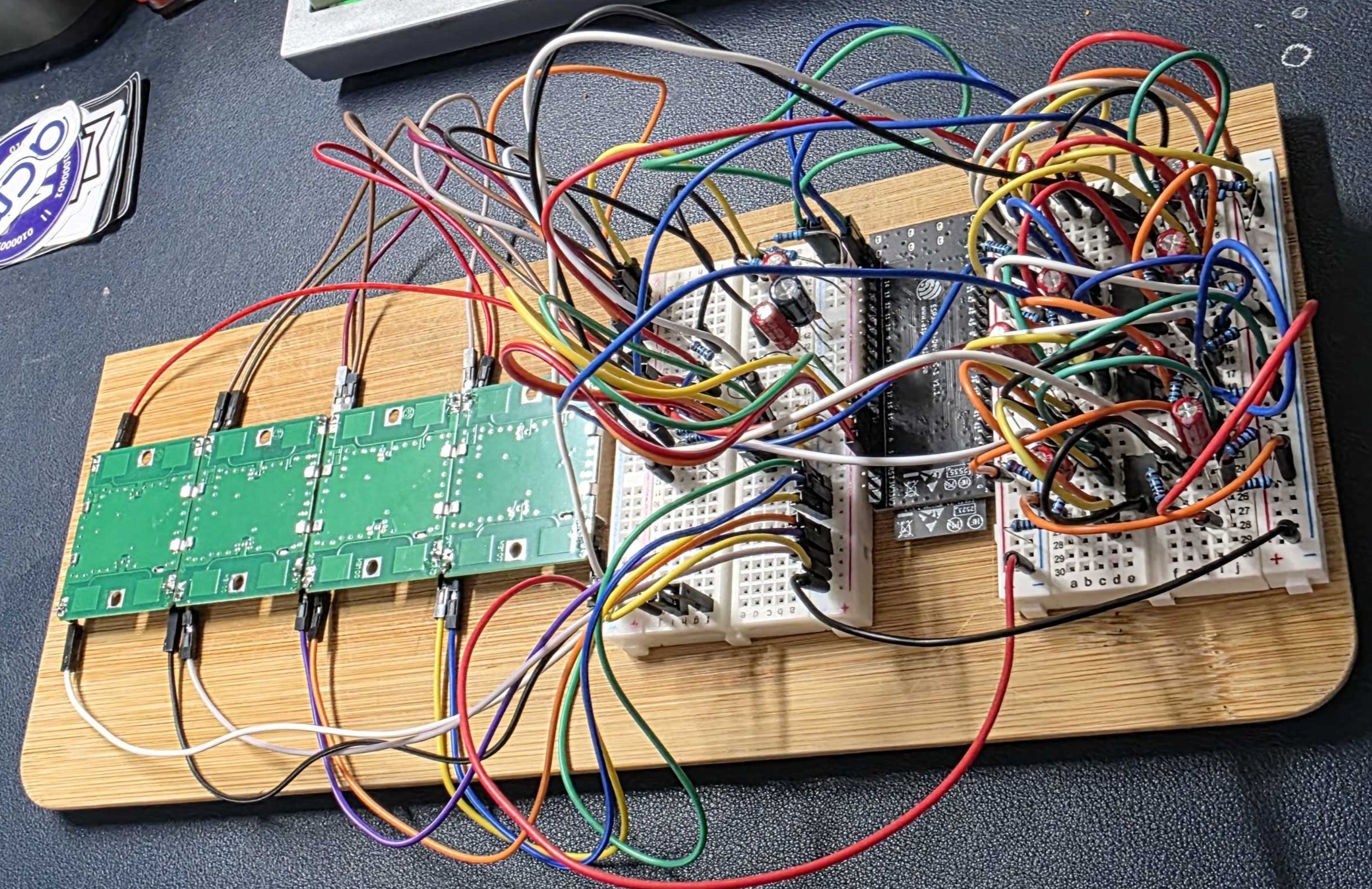
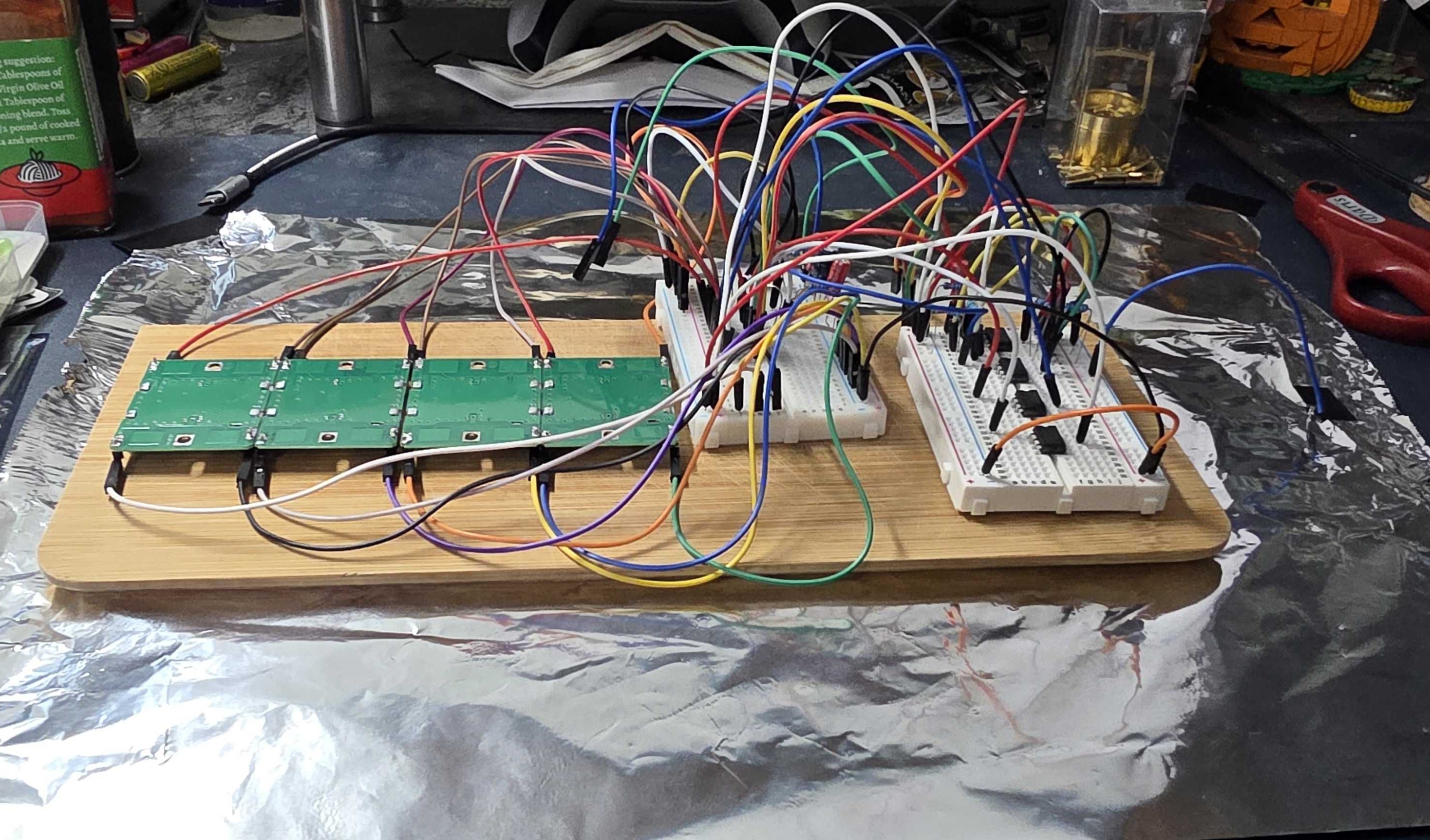
Circuit Photo - Breadboard Layout and Component Assembly
Electrostatic Discharge (ESD) Protected Area (EPA) - Lab Setup
Schema
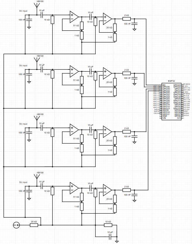
Signal Conditioning and Amplification Architecture
The HB100 IF output is inherently low-amplitude (10 µV to 2 mV range, typically at ~200 Hz nominal Doppler). The ESP32-S3 ADC (3.3 V rail, 12-bit, 0–4095 codes) cannot directly digitize negative-going signals without a DC reference offset. This constraint drives the three-stage analog front-end:
Stage 1: Virtual Ground Reference
Since the HB100 operates single-supply and its IF output can swing negative (relative to its GND), but the ESP32-S3 ADC input spans 0–3.3 V, a virtual ground at the midpoint of the ADC input range (1.65 V) is established using a resistive divider:
- Two matched resistors (10 kΩ each) connect the ESP32-S3's 3.3 V rail to GND
- The junction point (1.65 V) serves as the analog reference for the op-amp bias network
- This allows the ADC to "see" the full ±1.65 V swing around this midpoint, mapping the bipolar IF signal to the unipolar 0–3.3 V input range
Stage 2: First Op-Amp Stage (52× Gain, Non-Inverting Configuration)
A non-inverting amplifier using the MCP6002 provides a gain of (R_f / R_in) + 1:
- Input resistor: 1 kΩ
- Feedback resistor: 51 kΩ
- Gain = 51 + 1 = 52×
- Input is AC-coupled (1 µF capacitor) to remove DC offset before amplification
- Op-amp is biased around the virtual ground (1.65 V), allowing input swing from 1.65 V ± some fraction of the VCC range
Pre-amplifier EMI filtering:
- A low-pass filter (10 µF || 10 kΩ to virtual ground) is placed before this op-amp stage
- This filter attenuates environmental EMI (primarily at 50/60 Hz powerline and harmonics) with a cutoff frequency of ~1.6 Hz
- The 10 µF capacitor provides local energy storage; the 10 kΩ resistor to virtual ground sets the RC time constant
Stage 3: Second Op-Amp Stage (21× Gain, Inverting Configuration)
The inverted output of the first stage feeds the second op-amp (inverting amplifier):
- Input resistor: 1 kΩ
- Feedback resistor: 21 kΩ
- Gain = R_f / R_in = 21 / 1 = 21× (inverting, so output is 180° phase-shifted)
- This stage's output also references the virtual ground (1.65 V bias)
Total amplification: 52× × 21× = 1092× (60.8 dB)
Signal range at ADC input: The 10 µV–2 mV HB100 IF output is amplified and centered on the virtual ground (1.65 V):
- Minimum swing: 1.65 V − (2 mV × 1092) / 2 = 0.56 V
- Maximum swing: 1.65 V + (2 mV × 1092) / 2 = 2.74 V
- This maps to ADC codes ~683–5620 on the 0–4095 scale, utilizing ~66% of the full ADC range while staying safely within rail limits
Stage 4: Final Low-Pass Filter (Anti-Aliasing and EMI Rejection)
A single-pole RC filter at the ADC input:
- Resistor: 2 kΩ
- Capacitor: 100 nF
- Cutoff frequency: f_c = 1 / (2πRC) ≈ 796 Hz ≈ 800 Hz
- This filter is grounded to real GND (not virtual ground), providing final bandwidth limiting at the ADC input
- Rejects high-frequency noise and aliases above the Nyquist frequency (ADC sampling at 10 kHz, Nyquist = 5 kHz)
- Also prevents the op-amp's slewing and settling oscillations from entering the ADC
Electrostatic Discharge (ESD) Protected Area (EPA)
The MCP6002 op-amp is rated CMOS (JFET input stage) and highly susceptible to ESD damage. A simple but effective EPA was established using a single sheet of aluminum foil:
EPA Setup:
- A large sheet of aluminum foil (≥30 cm × 30 cm) was placed as a work surface on the breadboard area
- The foil was connected to the breadboard's GND rail via a wire or alligator clip (ensuring a direct, low-resistance path to circuit ground)
- Before any handling of op-amps: All power supplies to the circuit were disconnected (5V, 3.3V inputs isolated)
- Grounding procedure:
- Place both hands flat on the aluminum foil
- Maintain full skin contact for at least 3 seconds to allow body-to-foil charge equalization
- This drains accumulated static charge to ground (typically 5–10 kV potential) down to near-zero volts
- During op-amp handling: Both forearms remained in continuous contact with the aluminum foil at all times, maintaining a low-impedance path to ground
- This prevents any charge buildup during manipulation, soldering, or component insertion into the breadboard
Why this works:
- The human body can accumulate charge potentials of 1–15 kV under normal laboratory conditions (carpet movement, synthetic clothing, humidity gradients)
- The MCP6002's JFET input stage is damaged by discharges >100–200 V (gate-oxide breakdown)
- The aluminum foil (low resistivity, ~2.6 × 10⁻⁸ Ω·m) provides a high-conductance shunt path from body to circuit GND
- By keeping forearms in contact, any static buildup is continuously drained, reducing risk of sudden discharge during component insertion or pin contact
Additional EPA best practices applied:
- Work surface is clean and nonconductive (bamboo board atop foil avoids direct clothing-to-foil friction)
- No walking in and out of the EPA during sensitive work
- All conductors, solder joints, and IC pins are kept away from high-impedance floating nodes until the final assembly is complete
Power Supply Filtering (5V → 3.3V Path)
To stabilize the 5 V supply from the ESP32-S3's onboard regulator or external 5 V input feeding the MCP6002:
- Three 10 Ω resistors in parallel (effective ~3.3 Ω) in series with bulk capacitors
- Capacitor bank: 10 µF + 100 µF + 0.1 µF in parallel
- 100 µF: bulk, low-frequency filtering (10–100 Hz)
- 10 µF: mid-frequency (100 Hz–1 kHz)
- 0.1 µF: high-frequency transient decoupling (10 kHz and above)
- Resistors act as a current-limiting source and reduce inrush on power-up
Field-Deployable Antenna Array Layout
Hardware platform:
- Raspberry Pi 4 Model B (4 GB RAM) running host processor (Python)
- ESP32-S3-DevKitC-1 (dual core, 8 MB PSRAM, USB-CDC)
4-element linear ULA (Uniform Linear Array):
- Element 0 (farthest left): GPIO 7 (ADC1_CH6) @ 0.000 m → 37 mm to next
- Element 1: GPIO 6 (ADC1_CH5) @ 0.037 m → 38 mm to next
- Element 2: GPIO 5 (ADC1_CH4) @ 0.075 m → 37 mm to next
- Element 3 (closest/rightmost): GPIO 4 (ADC1_CH3) @ 0.112 m
Wavelength and DOA resolution:
- Carrier: f_c = 10.525 GHz
- Wavelength: λ = c / f_c ≈ 28.5 mm
- Max baseline: d_max = 112 mm ≈ 3.93 λ
- This baseline is sufficient for ±90° DOA coverage without aliasing (unambiguous range: ±sin⁻¹(λ / (2d)) ≈ ±sin⁻¹(0.128) ≈ ±7.4° per baseline)
- MUSIC pseudospectrum is computed over ±80° to cover most practical angles
Data flow:
HB100 #0 → 5V + GND → Analog conditioning → GPIO 7 (ADC1_CH6) → DMA → USB-CDC
HB100 #1 → 5V + GND → Analog conditioning → GPIO 6 (ADC1_CH5) → DMA → USB-CDC
HB100 #2 → 5V + GND → Analog conditioning → GPIO 5 (ADC1_CH4) → DMA → USB-CDC
HB100 #3 → 5V + GND → Analog conditioning → GPIO 4 (ADC1_CH3) → DMA → USB-CDC
         ↓
    Raspberry Pi 4
         ↓
        DSP
  (MUSIC or Monopulse)
         ↓
  Extended Kalman Filter Tracking
Signal Processing Pipelines
Radar Processor Pipeline (radar_processor.py)
The full-featured pipeline enabling phase-coherent angle-of-arrival estimation via MUSIC:
-
USB Serial Reception & Framing
- Scans incoming bytes for 0xDEADBEEF sync word (4 bytes)
- Reads sample count (4 bytes, uint32 LE, always 1024)
- Reads 1024 × 4 channels × 2 bytes (uint16 LE) raw ADC data
- Converts to float64 volts: V = (ADC_counts / 4095) × 3.3 V
-
DC Offset Removal
- Per-channel mean subtraction: centered[t, ch] = raw[t, ch] − mean(raw[:, ch])
- Removes low-frequency oscillator drift and DC biases from the virtual ground circuit
-
Bandpass Filtering (4th-order Butterworth)
- Low cutoff: 10 Hz (removes near-DC drifts)
- High cutoff: 800 Hz (matches hardware anti-alias filter; rejects out-of-band noise)
- Implementation: Second-Order-Sections (SOS) form for numerical stability
- Applied per-channel via
scipy.signal.sosfilt
-
Windowing and FFT
- Hanning window applied: windowed[t, ch] = filtered[t, ch] × hann(1024)[t]
- 1024-point real FFT per channel (rfft, taking advantage of conjugate symmetry)
- Output: 513 bins (DC to Nyquist, 0–5 kHz)
- Frequency resolution: 5000 Hz / 512 ≈ 9.77 Hz per bin
-
Peak Doppler Detection
- Compute average magnitude spectrum across all 4 channels: avg_mag[bin] = mean(|FFT_ch0|, ..., |FFT_ch3|)[bin]
- Identify peak bin (excluding DC): peak_bin = argmax(avg_mag[1:]) + 1
- Extract peak frequency and magnitude; compute SNR_dB = 20 log₁₀(peak_mag / noise_floor)
-
Phase Extraction at Peak Bin
- Extract complex FFT outputs at peak_bin for all channels
- Compute per-channel phase: phase[ch] = angle(FFT[peak_bin, ch])
-
Pairwise Phase Differences & Angle Estimation
- For each baseline (i, j) with spacing d_ij:
- Δφ_ij = phase[i] − phase[j] (wrapped to [−π, π])
- sin(θ) = (Δφ_ij × λ) / (2π × d_ij)
- θ_deg = arcsin(clipped sin(θ)) [clipped to [−1, +1] to handle aliasing]
- These 6 pairwise estimates provide redundant DOA candidates for diagnostic display
- For each baseline (i, j) with spacing d_ij:
-
MUSIC (MUltiple SIgnal Classification) for Refined Angle Estimation
- Form correlation matrix R from FFT bin range around peak (default: ±5 bins)
- R = (1/N) Σ x · x† (sum of outer products of complex FFT columns)
- Apply forward-backward averaging for real-valued symmetry: R ← 0.5(R + J·R*·J) where J = flip(I)
- Compute eigendecomposition: R = U·Λ·U†
- Noise subspace = eigenvectors corresponding to smallest eigenvalues (typically 3 out of 4)
- Pseudospectrum P(θ) = 1 / |E_noise† · a(θ)|² where a(θ) is the steering vector
- Peak in pseudospectrum ≈ true angle of arrival (within ±80° range)
- Form correlation matrix R from FFT bin range around peak (default: ±5 bins)
-
Speed Estimation
- Doppler frequency = f[peak_bin]
- Speed = (f_doppler × c) / (2 × f_carrier) where c = 3×10⁸ m/s, f_carrier = 10.525 GHz
- Factor of 2 accounts for round-trip (radar equation)
-
Extended Kalman Filter (EKF) Tracking
- State vector: x = [x_m, y_m, v_x, v_y] (2D position and velocity)
- Measurement vector: z = [range_m, angle_deg]
- Range is estimated from speed magnitude and track history; angle comes from MUSIC peak
- Predict step: x ← F·x (constant velocity motion model, dt = ~0.1 s per block)
- Update step: apply measurement residual with adaptive noise covariance tuning
- Output: filtered position and velocity estimates
Zone Classifier Pipeline (zone_classifier.py)
A simplified, LO-drift-robust alternative that omits phase processing entirely:
-
USB Serial Reception & DC Removal (identical to radar processor)
-
Bandpass Filtering (4th-order Butterworth, 10–800 Hz)
-
Windowing and FFT (identical Hanning window, 1024-point FFT)
-
Peak Doppler Detection (identical average spectrum method)
-
Amplitude-Based Monopulse DOA
- Per-channel gains (gain_factors[ch]) optionally applied to correct for hardware imbalances
- Corrected magnitudes: channel_mags[ch] = |FFT[peak_bin, ch]| × gain_factors[ch]
- Left/right bias: bias = (right_energy − left_energy) / (right_energy + left_energy)
- left_energy = channel_mags[0] + channel_mags[1]
- right_energy = channel_mags[2] + channel_mags[3]
- Resulting bias ∈ [−1, +1]: −1 ⟹ all on left; +1 ⟹ all on right
- Centroid estimate (weighted channel index): raw_centroid = Σ(channel_mags[ch] × ch) / Σ channel_mags
- Normalized to bias range: centroid_bias = (raw_centroid − 1.5) / 1.5
-
Zone Classification
- Bias is mapped to 5 zones via threshold-based lookup:
- FAR_LEFT: bias ≤ −0.50
- LEFT: −0.50 < bias ≤ −0.15
- CENTER: −0.15 < bias ≤ +0.15
- RIGHT: +0.15 < bias ≤ +0.50
- FAR_RIGHT: bias > +0.50
- Thresholds are empirically tuned against calibration targets at known angles
- Bias is mapped to 5 zones via threshold-based lookup:
-
Speed Tracking (1-D Alpha-Beta Filter)
- Scalar state: speed, acceleration
- Update with measured Doppler speed; predict forward when no detection
- Alpha weight (0.35) and beta weight (0.10) for smooth, responsive tracking
- Maintains 50-sample history deque for averaging or post-processing
-
Output
- Prints or logs: detected (true/false), zone, bias, speed, SNR, per-channel diagnostics
- CSV format: timestamp, zone, speed_mps, bias, snr_db, ch0_mag, ..., ch3_mag
Hardware Design Rationale
Why virtual ground?
The HB100 IF output is AC-coupled from an internal oscillator, with a nominal DC bias near GND (0 V). When the IF signal swings negative (relative to GND), a unipolar ADC (0–3.3 V input) cannot capture it. Biasing the op-amp's non-inverting input at 1.65 V (half the 3.3 V rail) allows the amplified signal to center on this midpoint, so negative swings (from the first stage's gain) map to 0–1.65 V and positive swings map to 1.65–3.3 V.
Why multi-stage op-amp gain?
The 10 µV–2 mV HB100 IF output is at the noise floor of a 12-bit ADC (LSB ≈ 0.8 mV). A single 1092× amplifier would require feedback resistors exceeding 1 MΩ, introducing thermal noise and stability issues. Splitting gain across two stages (52× + 21×) keeps component values practical (1–51 kΩ range) and improves slew rate and settling time performance.
Why 52× and 21× specifically?
These ratios (R_f / R_in = 51/1 and 21/1) are chosen to achieve ~1092× total gain while maintaining standard resistor values. The first stage's non-inverting topology preserves DC bias; the second stage's inverting topology inverts the signal (which is fine for Doppler processing, as only magnitude matters). Together, they yield good transient response and minimal phase distortion in the 10–800 Hz band.
Why the multi-capacitor power supply filter?
The MCP6002 op-amp requires clean, low-noise power. A single 10 µF or 100 µF capacitor resonates with parasitic inductance in typical PCB layouts, creating anti-resonances. Three capacitors in parallel (10 µF, 100 µF, 0.1 µF) span frequency ranges: 100 µF dominates at DC–10 Hz, 10 µF at 10–1 kHz, and 0.1 µF at 1–10 kHz, providing >50 dB attenuation across the audio band.
Why 800 Hz final cutoff?
Doppler shifts for targets moving at typical human walking speeds (1–2 m/s) or vehicle speeds (10–30 m/s) at 10.525 GHz produce shifts in the 70–700 Hz range. An 800 Hz cutoff captures the full Doppler band while rejecting powerline hum (50/60 Hz and harmonics, especially 100/120 Hz) and higher-frequency EMI from digital circuitry and switching supplies.
Deployment Notes
-
Calibration: Run
zone_classifier.py --calibrate --cal-blocks 100(no moving targets) to measure noise floor and compute per-channel gain factors. -
MUSIC requires phase coherence: Ensure HB100 modules have clean, isolated 5 V supplies and GND paths to minimize phase noise. Each HB100's Gunn oscillator is free-running, so low-frequency drift (<1 Hz) is acceptable, but high-frequency phase noise (>100 Hz) degrades MUSIC performance.
-
Cooling: HB100 and op-amp IC dissipate power. In extended operation, consider adding passive heatsinks or enforcing adequate ventilation to keep junction temperature below 85°C.
-
ESD precautions: The analog front-end is susceptible to electrostatic discharge (ESD) on unshielded traces. A proven low-cost EPA can be established using a sheet of aluminum foil connected to circuit GND; ground your body on the foil for 3+ seconds before handling op-amps, and keep forearms in contact with the foil during all component manipulation. See the Schema section for detailed EPA setup procedure.
-
Tuning for your environment: The ZONE_THRESHOLDS in
zone_classifier.pyand MUSIC parameters inradar_processor.pymay require adjustment for your particular array geometry, mounting orientation, and target profiles. Start with calibration and empirical angle sweeps.